Lag Features vs Rolling Windows For Sales Forecasts
Compare lag and rolling-window features for weekly sales forecasts; backtest all configurations with cutoff-safe walk-forward tests.


I use lags to track individual past weeks and rolling windows to smooth weekly noise. Start with last week’s sales and a 4-week average, using only completed weeks. Test each approach - and their combination - on the same future weeks before choosing a model.
Here’s what I check:
- Timing and seasonality: Lags 1, 4, 13, and 52 show past weekly sales. A 52-week lag needs about a year of history.
- Level and change: Rolling means, medians, totals, ranges, standard deviation, and growth measures show recent demand, volatility, and direction.
- Data quality: Keep sales definitions fixed, separate missing reports from zero sales, and <u>exclude the target week</u>.
- Forecast results: Compare lag-only, rolling-only, and combined models against simple baselines using walk-forward tests, MAE, RMSE, and WAPE.
- Outreach: Use authorized sales history to assess merchant growth. Keep StoreCensus estimates separate, and track outreach results apart from forecast error.
Quick Comparison
| Criterion | Lag features | Rolling windows |
|---|---|---|
| Input | One past week per lag | Several completed weeks |
| Best suited to | Recent changes and seasonal comparisons | Sales levels, noise, and volatility |
| Main trade-off | One unusual week can distort the signal | Longer windows react slowly to change |
| History needed | At least the selected lag | Enough weeks to fill the window |
My rule: choose the simplest approach that lowers holdout error. Better forecasts don’t automatically mean better outreach targets.
Creating Lag and Rolling Features for Time Series Analysis in Python
sbb-itb-61169e3
Lag Features vs Rolling Windows: Strengths and Limits
Lag Features vs Rolling Windows for Sales Forecasting
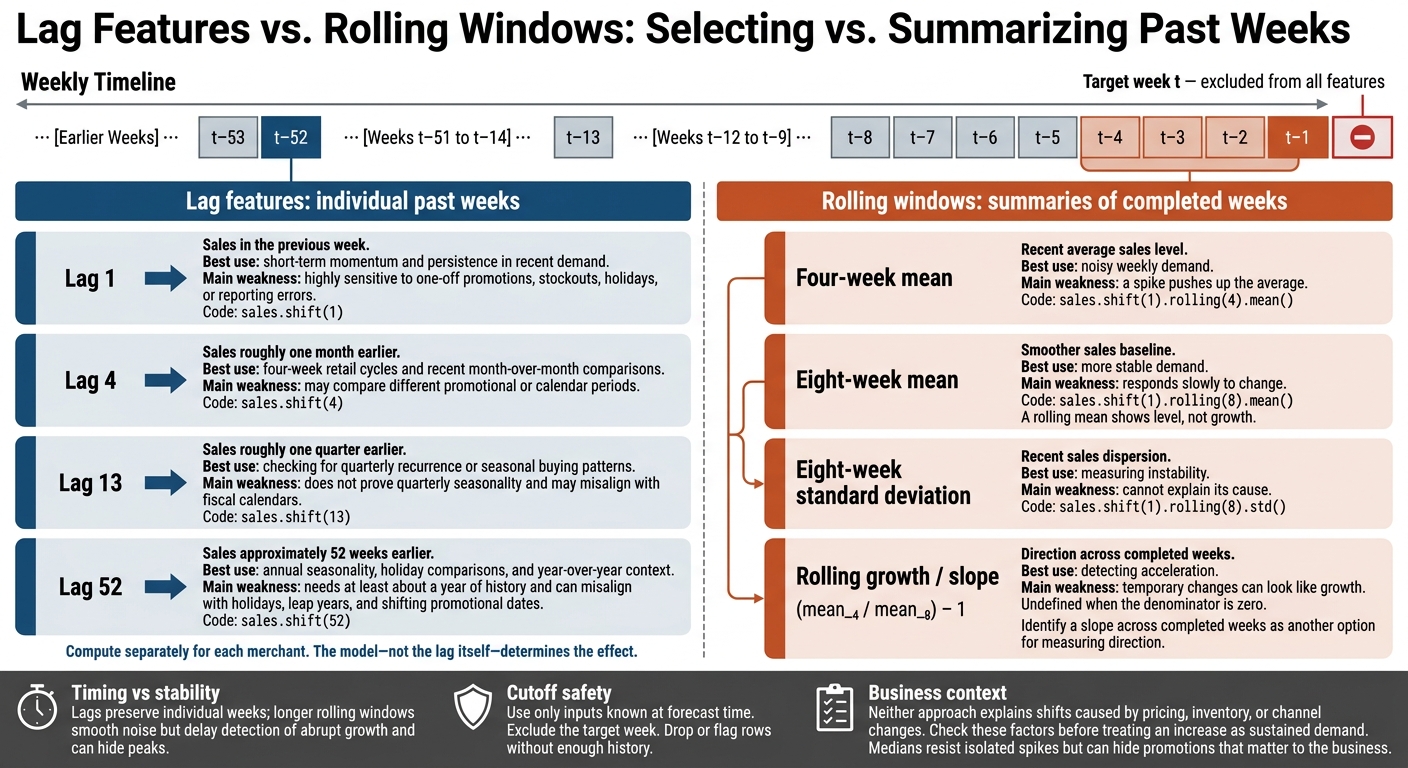
Each feature describes a different part of past demand. This table shows what it measures, when to use it, and where it can fall short.
| Feature | What it measures | Best use | Main weakness |
|---|---|---|---|
| Lag 1 | Sales in the previous week | Short-term momentum and persistence in recent demand | Highly sensitive to one-off promotions, stockouts, holidays, or reporting errors |
| Lag 4 | Sales roughly one month earlier | Four-week retail cycles and recent month-over-month comparisons | May compare different promotional or calendar periods |
| Lag 13 | Sales roughly one quarter earlier | Checking for quarterly recurrence or seasonal buying patterns | Does not prove quarterly seasonality and may misalign with fiscal calendars |
| Lag 52 | Sales approximately 52 weeks earlier | Annual seasonality, holiday comparisons, and year-over-year context | Needs at least about a year of history and can misalign with holidays, leap years, and shifting promotional dates |
| Four-week mean | Recent average sales level | Noisy weekly demand | A spike pushes up the average |
| Eight-week mean | Smoother sales baseline | More stable demand | Responds slowly to change |
| Eight-week standard deviation | Recent sales dispersion | Measuring instability | Cannot explain its cause |
| Rolling growth / slope | Direction across completed weeks | Detecting acceleration | Temporary changes can look like growth |
Lag Features Keep Individual Past Weeks
Sort the data by week, then compute sales.shift(1), sales.shift(4), and sales.shift(52) separately for each merchant. Apply the same forecast cutoff to every merchant. This consistency is vital when analyzing Shopify brand prospect lists for sales outreach. The model - not the lag itself - determines the effect.
A promotion can inflate a lag, while a stockout can push it down. Intermittent sales produce many zero-valued lags. Use only lagged inputs known at forecast time, and avoid piling on lag columns: too many can add noise and lead to overfitting.
Rolling Windows Summarize Sales Levels and Volatility
Use sales.shift(1).rolling(4).mean() and sales.shift(1).rolling(8).std() to exclude the target week from its own feature. Drop or flag rows without enough history. Medians resist isolated spikes; minimums and maximums preserve the recent range.
A rolling mean shows level, not growth. To measure trailing growth, use (mean_4 / mean_8) - 1, leaving the result undefined when the denominator is zero. Another option is to fit a slope across completed weeks.
Longer windows smooth noise, but they also delay detection of abrupt growth and hide peaks. Medians can hide promotions that matter to the business. Neither lags nor rolling summaries explain shifts caused by pricing, inventory, or channel changes. Check those factors before treating an increase as sustained demand.
Choose Features by Demand Pattern and Available History
| Demand pattern or history | Useful lag features | Useful rolling features | Main caution |
|---|---|---|---|
| Stable | Lags 1 and 4 | Four- and eight-week means; eight-week standard deviation | Small differences may be noise |
| Seasonal | Lags 13 and 52 | Thirteen-week mean; seasonal summaries | Test calendar and prior-year comparability. Treat this as a seasonality check, not proof. |
| Promotion-driven | Lag 1; promotion-specific lags where available | Median, maximum, standard deviation, promotion-aware means | Raw features can mistake campaign effects for baseline demand |
| Abrupt growth | Lags 1 and 4 | Four-week mean versus eight-week mean; slope | Older observations dilute the new level |
| Intermittent | Selected lags and nonzero-event indicators | Median, nonzero count, minimum, maximum, longer summaries | Ordinary means and zero-valued lags can obscure event timing |
| Short history | Only lags supported by available history | Short, complete windows | Do not use lag 13 or 52 without enough history |
Build clean backtests with these feature choices, using completed weeks only.
Build and Test Features Without Data Leakage
Use Completed Weeks and Consistent Sales Data
Once you’ve chosen lags and rolling windows, test them with cutoff-safe backtests: use only data available when each forecast would have been made.
Define one weekly sales measure in USD. Keep week boundaries, time zone, refunds, and tax/shipping treatment fixed. For example, net product sales can mean gross product sales minus discounts and refunds, excluding taxes and shipping. If refunds change earlier weeks, use the values available at each forecast cutoff - not today’s corrected totals.
Build a complete weekly calendar for each merchant or SKU. True no-sale weeks are zero; reporting gaps stay missing. Start with lags 1–4; seasonal lags of 13, 26, or 52 weeks when there’s enough history; four- and eight-week means; an eight-week standard deviation; and four- and thirteen-week totals. Require complete windows and flag unavailable history.
Measure growth by comparing the latest four completed weeks with the preceding, nonoverlapping four weeks. If the prior total is zero, leave growth blank and add a prior_zero flag, or use dollar change instead. For pre-close forecasts, shift both windows back one more week.
Test growth features separately from event controls known at the cutoff. Use only events known at that point, and keep post-hoc diagnostics out of the model. Never fill unavailable lags with later actual sales.
Backtest Lag-Only, Rolling-Only, and Combined Models
Use identical walk-forward splits, forecast horizons, model families, and eligible evaluation rows. Train before each forecast origin, predict, then move forward. Fit all preprocessing inside each training fold, and keep feature selection and tuning within the training data. Don’t use random splits. Forecasting: Principles and Practice describes this rolling-origin validation approach.[4] Repeat the comparison separately for each horizon.
| Feature configuration | Forecast horizon | Backtest period | Error metric | History requirement |
|---|---|---|---|---|
| Lag-only | 1 week | Same held-out weeks | MAE, RMSE, WAPE | 4 weeks; longer for seasonal lags |
| Rolling-only | 1 week | Same held-out weeks | MAE, RMSE, WAPE | 8 weeks |
| Combined | 1 week | Same held-out weeks | MAE, RMSE, WAPE | 8 weeks plus any selected seasonal lag |
| Last-week baseline | 1 week | Same held-out weeks | MAE, RMSE, WAPE | 1 week |
| Seasonal-naive baseline | 1 week | Same held-out weeks | MAE, RMSE, WAPE | 13 or 52 weeks, depending on the seasonality used |
Report errors by merchant, size band, and demand condition - not just across the portfolio. MAE shows the average dollar miss, while RMSE penalizes large misses more. WAPE is useful for aggregate demand, but percentage errors can be unstable for low-volume merchants. WAPE is undefined when total actual sales are zero.
Report eligible row counts and zero-sales periods alongside the results. Keep a final, untouched holdout for the selected configuration.
Use the best backtested feature set to score merchant growth before outreach.
Use Merchant Growth Signals to Guide Outreach
After backtesting, use the best mix of lag and rolling features to create a merchant-priority score for outreach.
Score Momentum, Sustained Growth, and Data Confidence
Use a growth-readiness score to prioritize outreach - not predict exact revenue. Build it only from authorized weekly sales history, with these weights: 30% momentum, 25% sustained trend, 20% consistency, 15% data confidence, and 10% service fit/timing.
Lag features show recent jumps and reversals. Rolling features help confirm whether growth holds up. Measure sustained growth through consecutive four-week comparisons.
For example, check whether each of the last three four-week windows exceeded the prior window.
Put each component on a 0–100 scale using documented caps or percentile ranks within similar merchant groups. Keep the components visible so reps can explain what drives the score.
Measure volatility relative to average sales. Check acceleration against promotions and known seasonality, and compare equivalent calendar periods when demand is seasonal. Before assigning priority, flag repeated zeros, reversals, stockouts, migrations, and tracking changes.
Set minimum thresholds for history and data completeness. Missing signals do not mean zero growth. Rescale unavailable components only under a documented rule, lower confidence, and send weak records to research. Otherwise, use a separate observable-signal score.
Find and Research Merchants With StoreCensus
Use StoreCensus to find likely Shopify and WooCommerce targets. Apply the sales-derived score only when authorized sales history is available. Filter by estimated revenue range, country, technology stack, theme, and growth signals.[5]
Keep revenue estimates separate from authorized weekly sales history. They are not audited financial results, and they should not feed calculated lag features, rolling statistics, or sales-derived scores.[6] Label records without authorized history “observable signals only.”
Verify the service need before surfacing decision-maker contacts. Keep fit and timing separate: a merchant may match your specialty but not be ready to buy. Revisit qualified accounts when tracked store changes give you a timely, evidence-based reason to reach out.
Set Outreach Priority Bands and Track Results
Turn scores into four outreach bands.
| Priority band | Supporting signals | Data concerns | Next action |
|---|---|---|---|
| High priority | Sustained positive growth, acceptable consistency, strong data confidence, and clear service fit | Confirm the latest completed week and any disruptions | Research the decision-maker, personalize outreach around the verified need, and test a timely campaign |
| Watchlist | Positive movement with high volatility, a recent reversal, or limited history | Check promotions, stockouts, seasonality, and history | Monitor the merchant, document the trigger, and reach out when the evidence is more stable |
| Low priority | Weak service fit, flat or declining demand without an addressable need, or too few supporting signals | Limited evidence or relevance | Deprioritize routine outreach, but retain the account if the agency can solve a clearly identified problem |
| Research required | Growth appears distorted by missing data, repeated zeros, disruptions, or conflicting public signals | Unresolved data definitions or reliability | Verify the data and business context before assigning a final priority |
Recalculate sales-derived components after each completed week, update observable signals from the source, and save score snapshots for auditing.
Track qualification, positive-reply, meeting, proposal, and close rates by priority band, along with time to close and closed-won revenue. Adjust weights based on outreach outcomes - not forecast accuracy alone. Compare lag-only, rolling-only, and combined rankings under similar outreach conditions.
Do not automatically exclude declining merchants. A verified conversion, retention, or technical problem can offer a stronger service opportunity than growth alone.
Conclusion: Combine Features and Measure Results
After testing each feature set, pick the simplest one that reduces holdout error. Use the combined model only if it beats both lag-only and rolling-only models in walk-forward tests at the same horizon.[7][8][9]
Before crediting feature changes for lift, check promotions, stockouts, and tracking changes.
The same growth evidence can help prioritize outreach instead of predicting sales. Use StoreCensus to find merchants worth researching, then confirm growth using authorized sales history before reaching out.
Review forecast error and outreach outcomes separately each month. Better forecasts don’t always mean better prospects. Use lag features for timing and rolling windows for stability, and judge both by their results.
FAQs
How do I choose rolling windows for seasonal sales?
Match your rolling window to the seasonal cycle you’re tracking. A 24- to 36-month window works best for spotting peak months, slow quarters, and longer-term growth patterns [1]. For short-term demand or SKU-level patterns, you’ll generally need at least 6 months to get a steady read [1][2].
Year-over-year comparisons often give you a clearer, more accurate picture than month-to-month comparisons because seasonal swings can skew the latter [3].
How do I use lags for multiweek forecasts without leakage?
Build lag features using only sales data available before the forecast horizon. Data leakage happens when your inputs include data from the period you’re trying to predict.
Shift historical sales data to create these lags. For a week-four forecast based on week-one data, exclude weeks two and three during both training and inference.
To validate the model, hold out a recent period and measure forecast error on that unseen data.
How can I validate growth scores before outreach?
Use a 100-point scoring model: weight firmographic fit at 60% and behavioral intent at 40%. Before you finalize your outreach list, review scores weekly using real-time signals, such as app installs, revenue changes, or theme updates.
Run controlled tests to compare conversion rates for signal-based segments with those for static lists. Then adjust your filters based on which signals consistently convert marketing-qualified leads (MQLs) into sales-qualified leads (SQLs).